Let’s face it, we live in a superficial world where people are constantly judged by their appearance. The multi-billion cosmetic industry wouldn’t exist if everyone feels confident in their own skin.
Being attractive is a valuable asset in the market. But how do we measure it?
In recent months, I spent a considerable amount of my time doing research about dating apps, which is the virtually perfect platform to measure the superficial traits of a person. Decisions are almost entirely based on looks. Whatever that is tied on the “Personality & Hobbies” section are merely a placebo. Words alone will not suffice when it comes to feeling attracted to a person.
The content that follows are based on my own formulation of an algorithm, which may or may not be used in current dating applications. Before I begin, please bear in mind that superficial qualities are inadequate when measuring one’s worth.
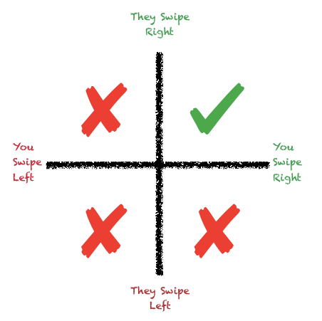
The process of installing and using dating apps is straightforward. It is a binary option & a match happens when 2 people like each other.
Algorithm #1
I obtained an inspiration parallel to the theory of correlation. Since it isn’t a binary concept, we could use a scale between -1 & 1 with 0 being the middle score.

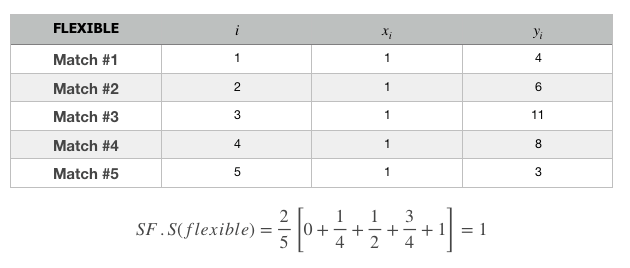
FLEXIBLE: Your matches rank you as their most appealing match
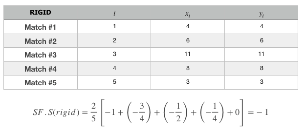
RIGID: Your matches rank you as their least appealing match
NEUTRAL: A mix of FLEXIBLE & RIGID
I uncovered a simple formula to calculate a person’s score on the scale above. I did a few tests and figured that it was quite accurate.
A user’s Superficial Score (SF.S) is as follows:

Note: If you have zero matches then the result will be ‘undefined’
Sample calculations can be found in the appendices section.
Algorithm #2
Before the results could be tabulated, the ranking parameter have to be defined. In other words, how are the matches being ranked for a particular user.
The ranking parameter is calculated as a score between 0 to 100%. Each user will have a distinct score and it will then be used to determine the ranking mentioned earlier
To make the ranking parameter as accurate as possible, factors such as “number of profiles swiped since the start” & “frequency of message replies from matches” should not influence the results.
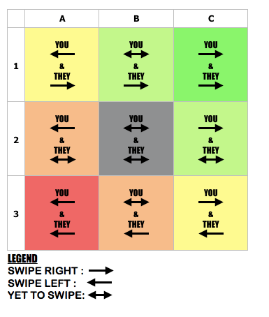
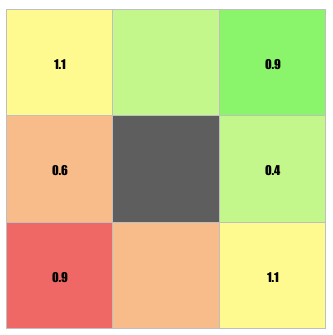
For every user, all the other people in the dating app can be categorised into 9 different groups as shown in the diagram below.
A user’s Rank Score (R.S) is given by: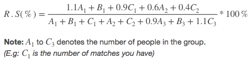
Further explanations with sample calculations can be found in the appendices section.
Summary
Time for a quick summary before diving to the appendices. If you’re feeling dizzy with all these numbers, hang in there just for a bit.
The main objective of this paper is to calculate the Superficial Score (SF.S) of a person via their dating app usage. This is done through the computation of Algorithm 1 which depends on the Rank Score(R.S) obtained from Algorithm 2. By incorporating advanced data analytical tools, the scores could be constantly updated & its fluctuation will be reduced as time goes by. It is a corollary to the rating of products in Amazon with the following statement. “The impact of your rating is inversely proportional to the total number of ratings for a particular product”
That’s all folks!
Appendices
Algorithm 1
Obtaining the possible scores
- To obtain the maximum score, one must be rated at the top for all their matches.
- To obtain the minimum score, one must be rated at the bottom for all their matches.
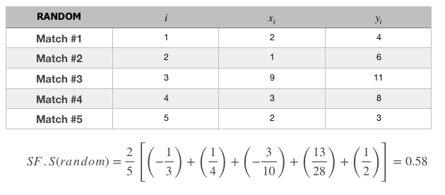
- To obtain a random score, one must be rated at random for all their matches.
Let’s apply the formula to the 3 types of people having the description above. We will use 5 matches for each of the 5 matches will have their own list of matches & this can be represented by the tables below.
Algorithm 2
 The derivation of the formula above is based on a two necessary concepts.
- The value of the middle grey box isn’t being used in the formula above because it represents the people you haven’t come across and vice versa.
- The multipliers indicated in the above figure is crucial. The comparisons will be explained further in the next section.
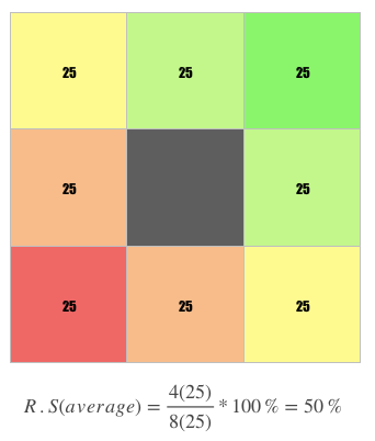
Next, I will explain the significance of all the multipliers. We can use a controlled environment of 200 people to test the validity of the multipliers. These 200 people will be categorised in 8 of the coloured groups in the figure above.
Before we begin making comparisons, we shall determine the baseline calculation of a the most average person, i.e, having equal distribution across the 8 groups.
Comparison #1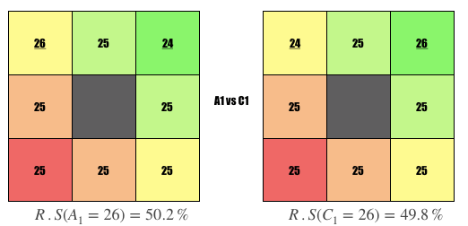
Question: Why is the user on the left ranked higher?
Answer: User is more picky, i.e., swipe left on 1 more person who already liked them.
Comparison #2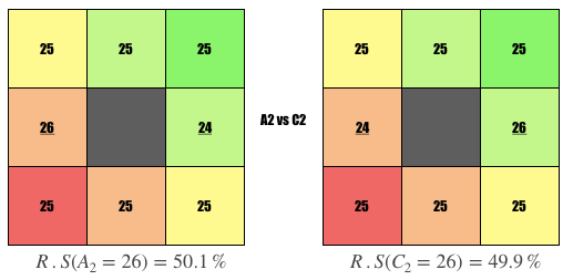
Question: Why is the user on the left ranked higher?
Answer: User is more picky, i.e., swipe left on 1 more person who hasn’t swiped on them.
Comparison #3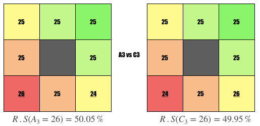
Question: Why is the user on the left ranked higher?
Answer: User is more picky, i.e., swipe left on 1 more person who disliked them.
Comparison #4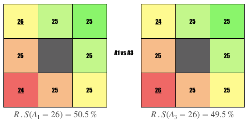
Question: Why is the user on the left ranked higher?
Answer: User is popular, i.e., liked by 1 more person whom they disliked
Comparison #5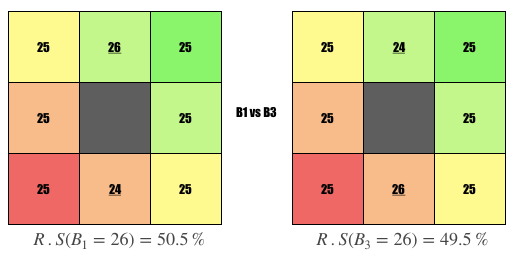
Question: Why is the user on the left ranked higher?
Answer: User is popular, i.e., liked by 1 more person whom they haven’t swiped
Comparison #6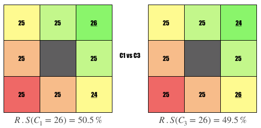
Question: Why is the user on the left ranked higher?
Answer: User is popular, i.e., liked by 1 more person whom they liked
From the 6 comparisons made above, we can conclude that the multipliers
are valid & it would provide a sound accuracy to the rank score.
With that, we have come to the end of the paper.
